Data Preparation Tutorial - Kidney Visium
Spatial-Live primarily centers around data visualization, with less emphasis on data processing. However, to effectively utilize Spatial-Live, it’s essential to supply appropriately formatted input files. This tutorial aims to illustrate the process of preparing these input files for the “A quick demo” showcased earlier. Specifically tailored to the 10X Visium platform, this demo serves as a valuable reference when configuring your own data visualization settings.
Python virtual environment setup
In order to run this Jupyter Notebook and streamline the process for your convenience, we have compiled several supplementary files including “requirements.txt”, which you can use to easily set up a Python virtual environment.
[1]:
# Please git clone the spatial-live from github,
# and change the WORKROOTDIR to your own working directory
%env WORKROOTDIR=/Users/zhenqingye/projects/spatial-live
env: WORKROOTDIR=/Users/zhenqingye/projects/spatial-live
[2]:
# You can use the below requirements.txt to create your virtual environment
! tree -L 1 ${WORKROOTDIR}/quickdemo/
/Users/zhenqingye/projects/spatial-live/quickdemo/
├── kidney
├── liver
└── requirements.txt
2 directories, 1 file
10X Visium spatial data preparation
The original data was downloaded from the kidney paper (GEO: GSM5224981), and we processed the raw data by the software tool Space Ranger from 10X website. The important outcomes have been saved in the “quickdemo/kidney” folder for our current purpose.
[3]:
! tree ${WORKROOTDIR}/quickdemo/kidney/
/Users/zhenqingye/projects/spatial-live/quickdemo/kidney/
└── Visium
└── outs
├── filtered_feature_bc_matrix.h5
└── spatial
├── aligned_fiducials.jpg
├── detected_tissue_image.jpg
├── scalefactors_json.json
├── tissue_hires_image.png
├── tissue_lowres_image.png
└── tissue_positions_list.csv
3 directories, 7 files
[4]:
import warnings
warnings.simplefilter('ignore')
import os
import numpy as np
import matplotlib.pyplot as plt
import scanpy as sc
import squidpy as sq
import pandas as pd
import PIL
pd.options.display.precision=3
sc.logging.print_header()
scanpy==1.9.5 anndata==0.9.2 umap==0.5.4 numpy==1.23.4 scipy==1.11.2 pandas==2.1.0 scikit-learn==1.3.0 statsmodels==0.14.0 igraph==0.10.8 pynndescent==0.5.10
Preprocessing and quality control
Again, please change the rootdir to your working directory accordingly.
[5]:
rootdir = "/Users/zhenqingye/projects/spatial-live/"
library_id = "Visium"
datadir = rootdir + 'quickdemo/kidney/'
[6]:
print(datadir)
/Users/zhenqingye/projects/spatial-live/quickdemo/kidney/
[7]:
adata = sc.read_visium(datadir + library_id + '/outs/', library_id=library_id)
adata.var_names_make_unique()
adata.obs.head(3)
[7]:
| in_tissue | array_row | array_col | |
|---|---|---|---|
| AAACAAGTATCTCCCA-1 | 1 | 50 | 102 |
| AAACACCAATAACTGC-1 | 1 | 59 | 19 |
| AAACAGCTTTCAGAAG-1 | 1 | 43 | 9 |
[8]:
adata.shape
[8]:
(1889, 32285)
[9]:
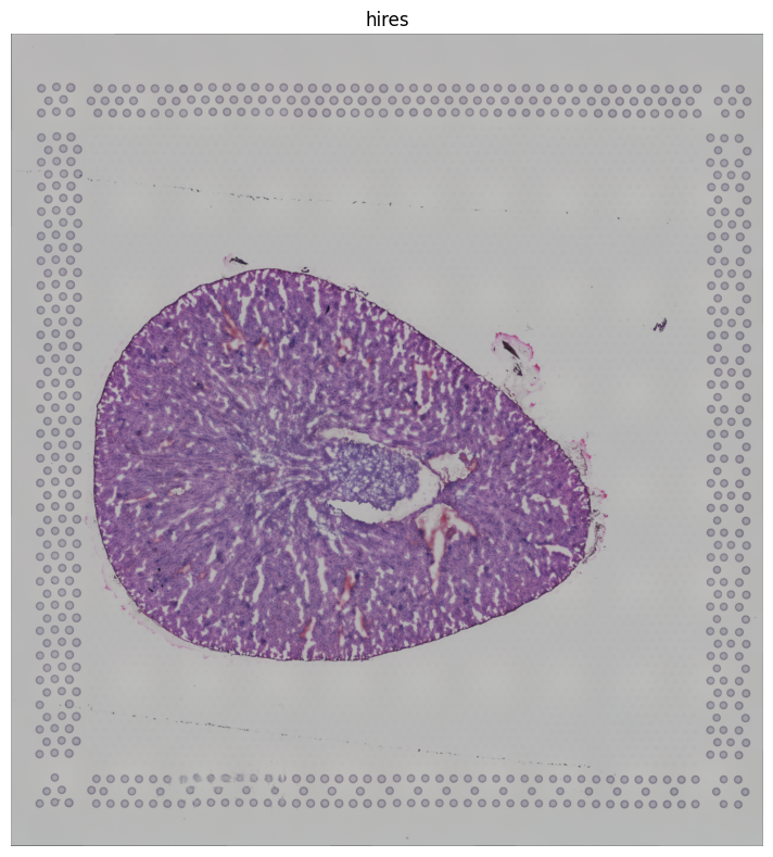
imgContainer = sq.im.ImageContainer.from_adata(adata)
imgContainer.show(layer='hires')
[10]:
adata.var["mt"] = adata.var_names.str.startswith('mt-')
sc.pp.calculate_qc_metrics(adata, qc_vars=["mt"], inplace=True)
sc.pl.violin(adata, ['n_genes_by_counts', 'total_counts', 'pct_counts_mt'], jitter=0.4, multi_panel=True, rotation=45)

[11]:
#keep in mind that here cells are actually spots
sc.pp.filter_cells(adata, min_genes=100, inplace=True)
sc.pp.filter_genes(adata, min_cells=10, inplace=True)
adata.shape
[11]:
(1889, 15634)
[12]:
adata.obs.head(3)
[12]:
| in_tissue | array_row | array_col | n_genes_by_counts | log1p_n_genes_by_counts | total_counts | log1p_total_counts | pct_counts_in_top_50_genes | pct_counts_in_top_100_genes | pct_counts_in_top_200_genes | pct_counts_in_top_500_genes | total_counts_mt | log1p_total_counts_mt | pct_counts_mt | n_genes | |
|---|---|---|---|---|---|---|---|---|---|---|---|---|---|---|---|
| AAACAAGTATCTCCCA-1 | 1 | 50 | 102 | 6206 | 8.733 | 37805.0 | 10.540 | 34.744 | 40.804 | 48.954 | 62.415 | 5914.0 | 8.685 | 15.643 | 6206 |
| AAACACCAATAACTGC-1 | 1 | 59 | 19 | 4693 | 8.454 | 20990.0 | 9.952 | 34.359 | 40.629 | 49.123 | 63.016 | 3089.0 | 8.036 | 14.717 | 4693 |
| AAACAGCTTTCAGAAG-1 | 1 | 43 | 9 | 5887 | 8.681 | 41463.0 | 10.633 | 34.428 | 41.357 | 50.397 | 65.058 | 3571.0 | 8.181 | 8.612 | 5887 |
[13]:
sc.pp.normalize_total(adata, target_sum=1e5, inplace=True)
sc.pp.log1p(adata)
Highly variable genes and leiden clustering
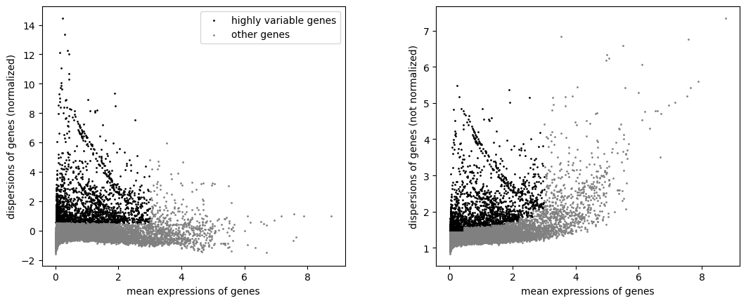
In this section, we will continue the classical analysis for this single-cell data, namely go through highly virable gene filtering, PCA dimention reduction, as well as leiden clustering.
[14]:
sc.pp.highly_variable_genes(adata, min_mean=0.0125, max_mean=3, min_disp=0.5)
sc.pl.highly_variable_genes(adata)
[15]:
#we will keep original data into the raw variable for future using
adata.raw = adata
[16]:
adata = adata[:, adata.var.highly_variable]
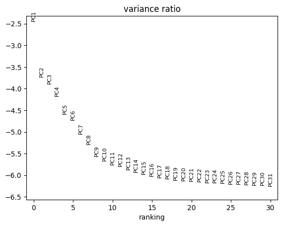
sc.pp.scale(adata, max_value=10)
sc.tl.pca(adata, svd_solver='arpack')
sc.pl.pca_variance_ratio(adata, log=True)
Dimensionality Reduction, Neighbor Calculation, and Clustering
[17]:
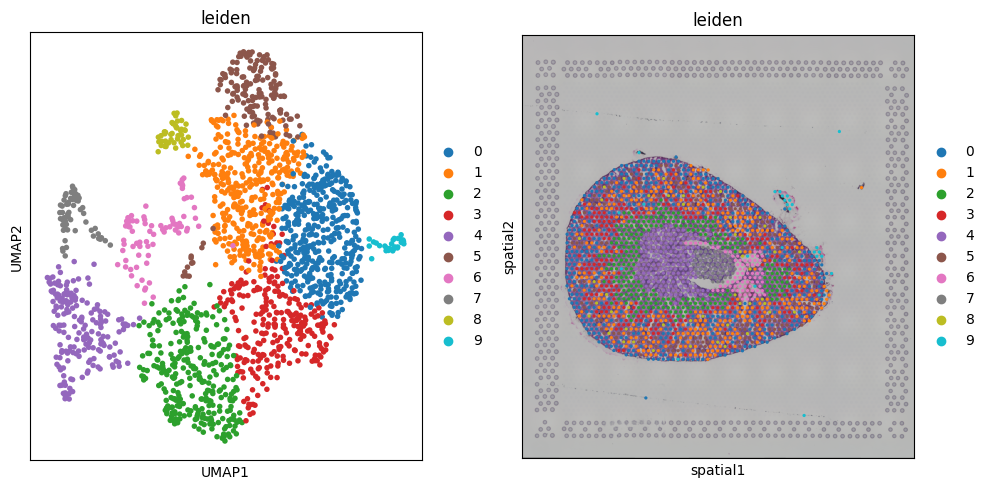
sc.pp.neighbors(adata, n_neighbors=10, n_pcs=12)
sc.tl.leiden(adata,resolution=0.5)
sc.tl.umap(adata)
[18]:
fig, axs = plt.subplots(1, 2, figsize=(10, 5))
sc.pl.umap(adata, color='leiden', ax=axs[0], show=False)
sq.pl.spatial_scatter(adata, color=['leiden'], ax=axs[1])
fig.tight_layout()
Finding marker genes
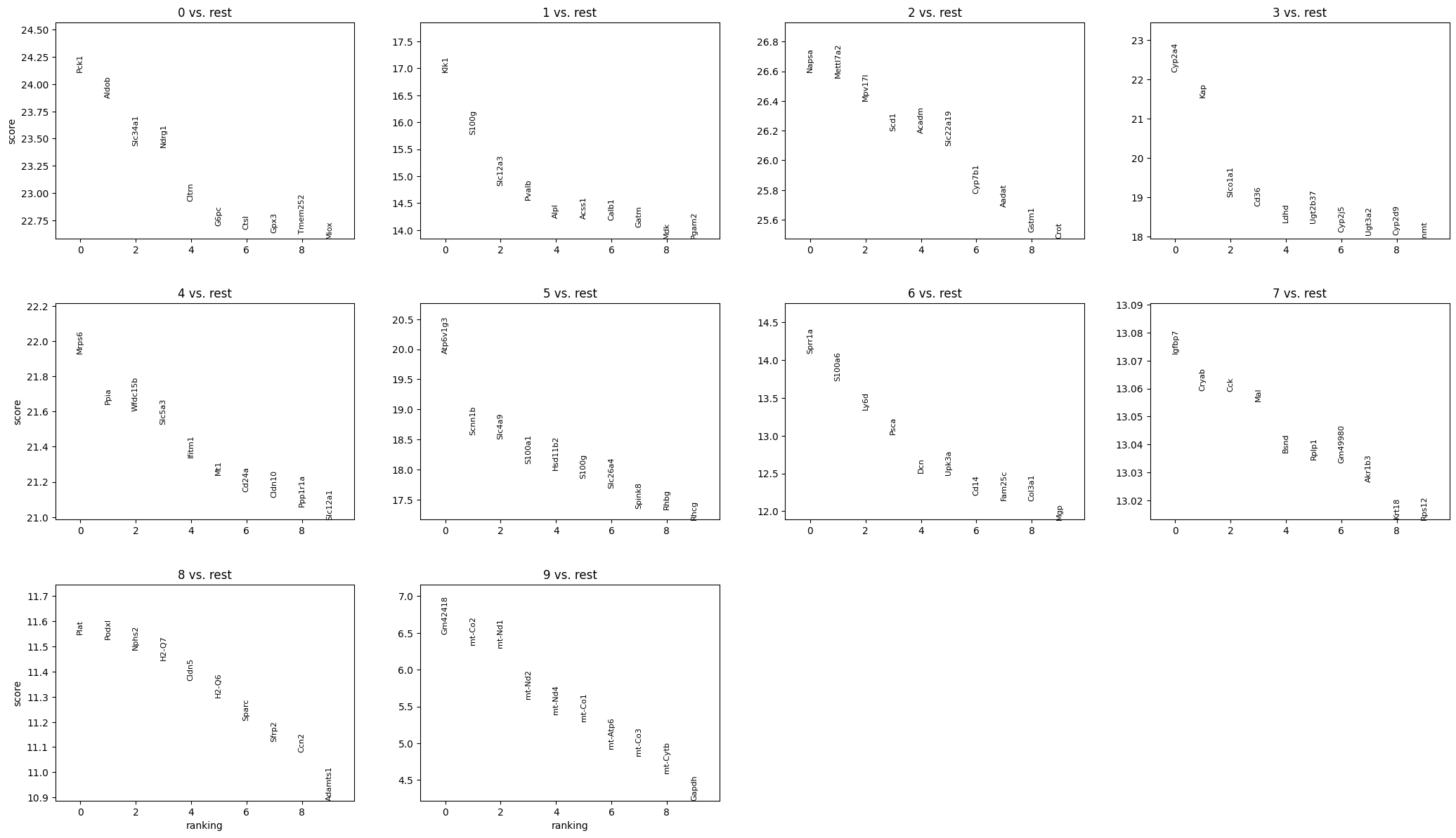
We will proceed to calculate a ranking for highly differential genes within each leiden group.
[19]:
sc.tl.rank_genes_groups(adata, groupby="leiden", method='wilcoxon')
sc.pl.rank_genes_groups(adata, n_genes=10, sharey=False)
[20]:
pd.DataFrame(adata.uns['rank_genes_groups']['names']).head(10)
[20]:
| 0 | 1 | 2 | 3 | 4 | 5 | 6 | 7 | 8 | 9 | |
|---|---|---|---|---|---|---|---|---|---|---|
| 0 | Pck1 | Klk1 | Napsa | Cyp2a4 | Mrps6 | Atp6v1g3 | Sprr1a | Igfbp7 | Plat | Gm42418 |
| 1 | Aldob | S100g | Mettl7a2 | Kap | Ppia | Scnn1b | S100a6 | Cryab | Podxl | mt-Co2 |
| 2 | Slc34a1 | Slc12a3 | Mpv17l | Slco1a1 | Wfdc15b | Slc4a9 | Ly6d | Cck | Nphs2 | mt-Nd1 |
| 3 | Ndrg1 | Pvalb | Scd1 | Cd36 | Slc5a3 | S100a1 | Psca | Mal | H2-Q7 | mt-Nd2 |
| 4 | Cltrn | Alpl | Acadm | Ldhd | Ifitm1 | Hsd11b2 | Dcn | Bsnd | Cldn5 | mt-Nd4 |
| 5 | G6pc | Acss1 | Slc22a19 | Ugt2b37 | Mt1 | S100g | Upk3a | Rplp1 | H2-Q6 | mt-Co1 |
| 6 | Ctsl | Calb1 | Cyp7b1 | Cyp2j5 | Cd24a | Slc26a4 | Cd14 | Gm49980 | Sparc | mt-Atp6 |
| 7 | Gpx3 | Gatm | Aadat | Ugt3a2 | Cldn10 | Spink8 | Fam25c | Akr1b3 | Sfrp2 | mt-Co3 |
| 8 | Tmem252 | Mdk | Gstm1 | Cyp2d9 | Ppp1r1a | Rhbg | Col3a1 | Krt18 | Ccn2 | mt-Cytb |
| 9 | Miox | Pgam2 | Crot | Inmt | Slc12a1 | Rhcg | Mgp | Rps12 | Adamts1 | Gapdh |
Preparing input files for Spatial-Live
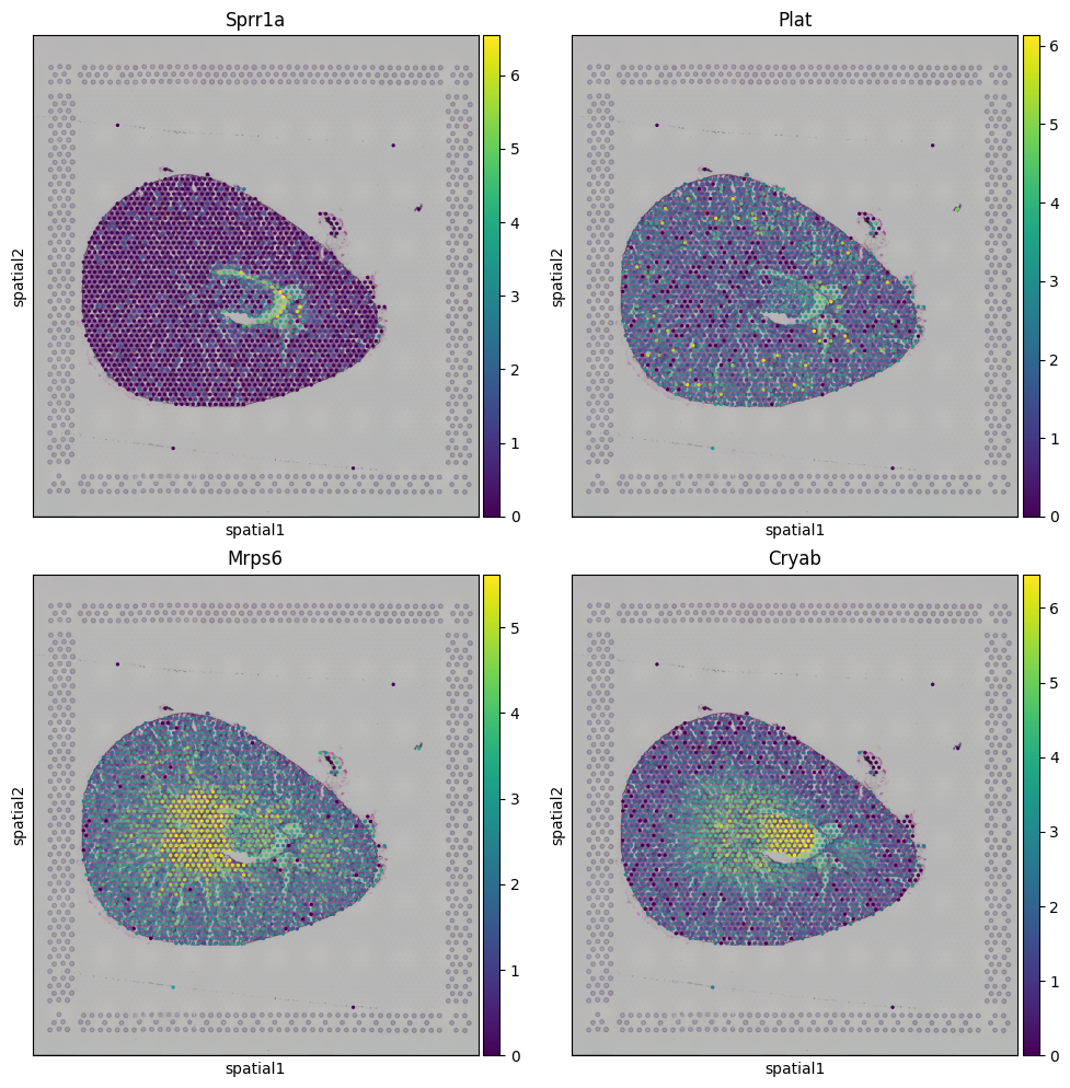
In this section, we prepare the necessary data columns for the Spatial-Live input CSV file. This includes a core set of columns, namely “id:barcode”, “pos:pixel_x” and “pos:pixel_y”. Additionally, we aim to incorporate several supplementary variables:
A categorical variable labeled “char:leiden”.
Two numerical variables: “num:Sprr1a” (representing the top gene from leiden-6 group) and “num:Plat” (representing the top gene from leiden-8 group).
Two gene variabels: “gene:Cryab” (the second-highest gene from leiden-7 group) and “gene:Mrps6” (representing the top gene from leiden-4 group) for heatmap plotting.
While gene variable data is inherently numerical, it undergoes a slightly different data processing approach in Spatial-Live, distinguishing it from standard numerical variables and warranting a distinct mention.
[21]:
fig, axs = plt.subplots(2, 2, figsize=(10, 10))
sq.pl.spatial_scatter(adata, color=['Sprr1a'], ax=axs[0,0], use_raw=True)
sq.pl.spatial_scatter(adata, color=['Plat'], ax=axs[0,1], use_raw=True)
sq.pl.spatial_scatter(adata, color=['Mrps6'], ax=axs[1,0], use_raw=True)
sq.pl.spatial_scatter(adata, color=['Cryab'], ax=axs[1,1])
fig.tight_layout()
We can extract these values from adata object now
[22]:
csv_out_df = sc.get.obs_df(adata, keys=['leiden', 'Sprr1a', 'Plat', 'Mrps6', 'Cryab'], use_raw=True)
csv_out_df.head(3)
[22]:
| leiden | Sprr1a | Plat | Mrps6 | Cryab | |
|---|---|---|---|---|---|
| AAACAAGTATCTCCCA-1 | 1 | 1.293 | 2.971 | 2.826 | 2.449 |
| AAACACCAATAACTGC-1 | 1 | 1.752 | 2.728 | 3.212 | 0.000 |
| AAACAGCTTTCAGAAG-1 | 3 | 0.000 | 1.227 | 2.365 | 1.762 |
To extract the positions of each cell (spot) in pixel space, it’s crucial to be mindful of the image employed. In our scenario, we exclusively use the “hires” version of the image for all preceding visualizations. As a result, we will persist in utilizing the “hires” image to compute the pixel positions of each cell. Additionally, it’s essential to account for disparities in the origin points (left, up) between the image coordinate system and the Spatial-Live pixel coordinate system (left, bottom).
[23]:
hires_sf = adata.uns['spatial'][library_id]['scalefactors']['tissue_hires_scalef']
hires_maxY = imgContainer.shape[0]
csv_out_df['pixel_x'] = adata.obsm['spatial'][:,0] * hires_sf
# csv_out_df['pixel_y'] = adata.obsm['spatial'][:,1] * hires_sf
# translate the origin point (Y-axis) to be consistent with the spatial-lvv pixel coordinate
csv_out_df['pixel_y'] = hires_maxY - adata.obsm['spatial'][:,1] * hires_sf
csv_out_df.head(3)
[23]:
| leiden | Sprr1a | Plat | Mrps6 | Cryab | pixel_x | pixel_y | |
|---|---|---|---|---|---|---|---|
| AAACAAGTATCTCCCA-1 | 1 | 1.293 | 2.971 | 2.826 | 2.449 | 1392.051 | 750.288 |
| AAACACCAATAACTGC-1 | 1 | 1.752 | 2.728 | 3.212 | 0.000 | 421.528 | 569.532 |
| AAACAGCTTTCAGAAG-1 | 3 | 0.000 | 1.227 | 2.365 | 1.762 | 305.391 | 895.105 |
And we further change the column names to comply with the rules from Spatial-Live, refer to the documents.
[24]:
csv_out_df.rename(columns={
"leiden": "char:leiden",
"Sprr1a": "num:Sprr1a",
"Plat": "num:Plat",
"Mrps6": "gene:Mrps6",
"Cryab": "gene:Cryab",
"pixel_x": "pos:pixel_x",
"pixel_y": "pos:pixel_y"
}, inplace=True)
csv_out_df.head(3)
[24]:
| char:leiden | num:Sprr1a | num:Plat | gene:Mrps6 | gene:Cryab | pos:pixel_x | pos:pixel_y | |
|---|---|---|---|---|---|---|---|
| AAACAAGTATCTCCCA-1 | 1 | 1.293 | 2.971 | 2.826 | 2.449 | 1392.051 | 750.288 |
| AAACACCAATAACTGC-1 | 1 | 1.752 | 2.728 | 3.212 | 0.000 | 421.528 | 569.532 |
| AAACAGCTTTCAGAAG-1 | 3 | 0.000 | 1.227 | 2.365 | 1.762 | 305.391 | 895.105 |
Now we will output the image (png file) and formated data sheet (csv file) to the target folder, which can be accessed from the Spatial-Live visualization tool.
[25]:
! mkdir -p ${WORKROOTDIR}/quickdemo/kidney/output
[26]:
img = np.squeeze(imgContainer['hires'])
img = PIL.Image.fromarray((img.to_numpy()*255).astype('uint8'))
img.save(datadir + "output/kidney_demo.png")
[27]:
csv_out_df.to_csv(datadir + "output/kidney_demo.csv", index_label="id:spot", float_format='%.3f')
[28]:
! tree ${WORKROOTDIR}/quickdemo/kidney/
/Users/zhenqingye/projects/spatial-live/quickdemo/kidney/
├── Visium
│ └── outs
│ ├── filtered_feature_bc_matrix.h5
│ └── spatial
│ ├── aligned_fiducials.jpg
│ ├── detected_tissue_image.jpg
│ ├── scalefactors_json.json
│ ├── tissue_hires_image.png
│ ├── tissue_lowres_image.png
│ └── tissue_positions_list.csv
└── output
├── kidney_demo.csv
└── kidney_demo.png
4 directories, 9 files
Notice that the two files (kidney_demo.csv and kidney_demo.png) have been stored in the “output” folder. And here we also briefly check the header and a few first rows in the kidney_demo.csv as below to see if it is compatible with the requirement from Spatial-Live.
[29]:
! head ${WORKROOTDIR}/quickdemo/kidney/output/kidney_demo.csv
id:spot,char:leiden,num:Sprr1a,num:Plat,gene:Mrps6,gene:Cryab,pos:pixel_x,pos:pixel_y
AAACAAGTATCTCCCA-1,1,1.293,2.971,2.826,2.449,1392.051,750.288
AAACACCAATAACTGC-1,1,1.752,2.728,3.212,0.000,421.528,569.532
AAACAGCTTTCAGAAG-1,3,0.000,1.227,2.365,1.762,305.391,895.105
AAACAGGGTCTATATT-1,1,0.000,3.311,3.006,2.361,351.952,813.667
AAACCGGGTAGGTACC-1,2,1.200,1.730,3.859,3.996,527.397,914.933
AAACCGTTCGTCCAGG-1,2,0.000,1.763,2.630,3.830,690.626,711.162
AAACCTCATGAAGTTG-1,2,0.000,1.385,4.247,2.771,422.413,1016.907
AAACGAGACGGTTGAT-1,1,1.642,2.602,3.407,1.642,1123.838,1056.033
AAACTGCTGGCTCCAA-1,7,4.083,3.258,3.932,5.884,983.093,852.970
Geometric Json file
In the following step, we’ll focus on generating the geometric JSON file. While this file is not mandatory for Spatial-Live, it can prove advantageous in certain scenarios. For instance, it comes in handy when annotating regions of interest (ROIs) on the image. For the more details, please refer to GeoJson specification. Within the “properties” section, each feature necessitates two key attributes: “id” and “group.” It’s worth noting that multiple JSON files are supported, and they should all be placed in the designated “json” folder.
[30]:
import holoviews as hv
from holoviews import opts, streams
from PIL import Image
import geojson
hv.extension('bokeh')
[31]:
img_uri = rootdir + 'quickdemo/kidney/Visium/outs/spatial/tissue_hires_image.png'
imarray = np.array(Image.open(img_uri).convert('RGBA'))
imarray.shape
[31]:
(2000, 1853, 4)
[32]:
IMG_HEIGHT, IMG_WIDTH = imarray.shape[0:2]
#flip to be consistent with the spatial-live coordinates
imarray = np.flip(imarray, axis=0)
hvimg = hv.RGB(imarray, bounds=(0, 0, IMG_WIDTH, IMG_HEIGHT))
Simple geometric polygons for JSON layer
During an active Jupyter server session, we have the capability to both edit and extract these polygons. However, in the context of a static HTML Sphinx document, the interactive real-time extraction of these polygons is not feasible. As a result, we have preconfigured these simple polygons and hardcoded them in this notebook for the sake of reproducibility and demonstration.
[33]:
# notice that the origin of the image in Bokeh plot is different from the origin in spatial-live coordinates,
# Therefore we need to transform it a little bit here to make them consistent
pg1 = {'x': np.array([381.96, 343.73, 622.3]), 'y': IMG_HEIGHT - np.array([760.15, 952.1, 923.95]) }
pg2 = {'x': np.array([803.69, 785.31, 960.61, 975.25, 921.99]), 'y': IMG_HEIGHT - np.array([872.77, 1002.79,965.38, 866.29, 832.04]) }
pg3 = {'x': np.array([1042.96, 1012.11, 1160.95, 1153.65]), 'y': IMG_HEIGHT - np.array([1043.75, 1189.68, 1132.59, 998.19]) }
mypolys = hv.Polygons([pg1, pg2, pg3])
#mypolys = hv.Polygons([])
[34]:
# need to be set before poly_stream
poly_edit = streams.PolyEdit(source=mypolys, vertex_style={'color': 'red'}, shared=True)
poly_stream = streams.PolyDraw(source=mypolys, drag=True, num_objects=4,
show_vertices=True, styles={
'fill_color': ['red', 'green', 'blue']
})
layout = hvimg * mypolys
layout.opts(
opts.Polygons( fill_alpha=0.4, height=500, width=500 ),
opts.RGB(height=500, width=500),
)
[34]: